OPTICS Benchmark

Test data for benchmarks

For these benchmarks I’m going to use real data– the data is heterogeneous, large, and publicly available. More specifically, the benchmark data is a set of ~8.5 million filtered LiDAR data points, collected by the National Ecological Observation Network (NEON) in 2013 over the D17 study domain site. More information about the field campaign and data can be found here. The data is spread over a rectangle that is slightly larger than a kilometer and half North/South by 0.75 kilometers East/West. A (very) coarse view of the of the points is shown below, with arbitrary units of relative density:

For these benchmarks (and for the plot above), I have filtered out the ground points; the remaining unstructured three-dimensional points are randomly dispersed vegetation clumps– mostly trees of various sizes, but also some bushes. An ideal clustering of this data set would resolve individual trees (or bushes) as objects.

The filtered data set for these benchmarks is available here for those wishing to run their own benchmarks. I’ll be using X, Y, Z locations for OPTICS and DBSCAN, but there are 10 dimensions included in the data set (additional spectral data from simultaneously flown spectroradiometer) for those curious about how the clustering performs in higher dimensional space. As the Jake Vanderplas has already documented and benchmarked higher dimensional search trees, these benchmarks will focus on only the three dimensional case, and will vary the epsilon and min samples parameters instead.

The main comparison here is between the OPTICS and DBSCAN algorithms when given identical input parameters and data. The two clustering approaches give nearly identical results with the same input parameters, so we will only be looking at runtime. DBSCAN will (or at least should) always be faster than OPTICS, and for small datasets will in fact be much faster– for this reason, the data set here is purposely large, as a practical use of the OPTICS algorithm is for large data sets where multiple cluster extraction a varying epsilons is desired (more detail on this point is described in the narrative documentation of OPTICS).

%pylab inline

Populating the interactive namespace from numpy and matplotlib

cd '~/Software/scikit-learn/'

/Users/grigsbye/Software/scikit-learn

from sklearn.externals import joblib
from sklearn.cluster import DBSCAN
from sklearn.cluster.optics import OPTICS

Testing Data

import pandas as pd # For test data

# This dataset is availible at:
# http://cires1.colorado.edu/shane/extractionLAS_subset.hdf
data = pd.HDFStore('/Users/grigsbye/Desktop/Tasha/extractionLAS_subset.hdf', 'r')
subset = data['subset']
len(subset)

8505072

# Trivial / small
subset4k = subset[(subset.X[:] > 256450) &
                  (subset.X[:] < 256455) &
                  (subset.Y[:] > 4110525) &
                  (subset.Y[:] < 4110575)]
len(subset4k) # 5 by 50 meters

4183

xyz4k = np.ones((len(subset4k),3))
xyz4k[:,0],xyz4k[:,1],xyz4k[:,2] = subset4k.X[:],subset4k.Y[:],subset4k.Z[:]

# Medium
subset40k = subset[(subset.X[:] > 256440) &
                   (subset.X[:] < 256460) &
                   (subset.Y[:] > 4110500) &
                   (subset.Y[:] < 4110600)]
len(subset40k) # 20 by 100 meters

41624

xyz40k = np.ones((len(subset40k),3))
xyz40k[:,0],xyz40k[:,1],xyz40k[:,2] = subset40k.X[:],subset40k.Y[:],subset40k.Z[:]

# Large ... this crashes DBSCAN at large epsilons
subset400k = subset[(subset.X[:] > 256200) &
                    (subset.X[:] < 256700) &
                    (subset.Y[:] > 4110500) &
                    (subset.Y[:] < 4110600)]
len(subset400k) # 500 by 100 meters

398359

xyz400k = np.ones((len(subset400k),3))
xyz400k[:,0],xyz400k[:,1],xyz400k[:,2] = subset400k.X[:],subset400k.Y[:],subset400k.Z[:]

# BIG ... not used, but included for the curious
subset4000k = subset[(subset.X[:] > 256250) &
                     (subset.X[:] < 256650) &
                     (subset.Y[:] > 4109500) &
                     (subset.Y[:] < 4111000)]
len(subset4000k) # 400 by 1500 meters

3978624

xyz4000k = np.ones((len(subset4000k),3))
xyz4000k[:,0],xyz4000k[:,1],xyz4000k[:,2] = subset4000k.X[:],subset4000k.Y[:],subset4000k.Z[:]

# Setting up benchmarks
# Taken from Jake Vanderplas
# https://jakevdp.github.io/blog/2013/04/29/benchmarking-nearest-neighbor-searches-in-python/
from time import time

def average_time(executable, *args, **kwargs):
    """Compute the average time over N runs"""
    N = 3
    t = 0
    for i in range(N):
#        print(i)
        t0 = time()
        res = executable(*args, **kwargs)
        t1 = time()
        t += (t1 - t0)
    return res, t * 1. / N

nsample = [5,10,20,50,100,150,200,250,500]
len(nsample)

9

epsilons = [0.15,0.3,0.6,1.2,2.5,5.0,10.0,20.0,50.0,100.0,250.0]
len(epsilons)

11

# Varying eps benchmark
eps_times_DB = []
eps_times_OPT = []
for epsilon in epsilons:
    benchmark_dbscan = DBSCAN(eps=epsilon, min_samples=100)
    outputDB = average_time(benchmark_dbscan.fit,xyz4k)
    eps_times_DB.append(outputDB[1])

    benchmark_cluster = OPTICS(eps=epsilon, min_samples=100)
    outputOPT = average_time(benchmark_cluster.fit,xyz4k)
    eps_times_OPT.append(outputOPT[1])

    print epsilon

0.15
0.3
0.6
1.2
2.5
5.0
10.0
20.0
50.0
100.0
250.0

# Varying samples benchmark
eps_times_DB_ = []
eps_times_OPT_ = []
for nsamples in nsample:
    benchmark_dbscan = DBSCAN(eps=5.0, min_samples=nsamples)
    outputDB = average_time(benchmark_dbscan.fit,xyz4k)
    eps_times_DB_.append(outputDB[1])

    benchmark_cluster = OPTICS(eps=5.0, min_samples=nsamples)
    outputOPT = average_time(benchmark_cluster.fit,xyz4k)
    eps_times_OPT_.append(outputOPT[1])

    #print nsamples

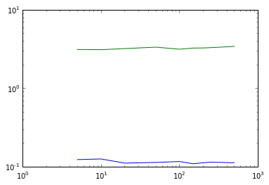
# Varying min_points plot
plot(nsample,eps_times_DB_,'b')
plot(nsample,eps_times_OPT_,'g')
semilogy()
semilogx()

[]

Note: Because of both long run times, and crashes with DBSCAN, some cells below were run on previous iPython kernels, and cell numbering is not

# Varying eps benchmark
eps_times_DB_40k = []
eps_times_OPT_40k = []
for epsilon in epsilons:
    benchmark_dbscan = DBSCAN(eps=epsilon, min_samples=100)
    outputDB = average_time(benchmark_dbscan.fit,xyz40k)
    eps_times_DB_40k.append(outputDB[1])

    benchmark_cluster = OPTICS(eps=epsilon, min_samples=100)
    outputOPT = average_time(benchmark_cluster.fit,xyz40k)
    eps_times_OPT_40k.append(outputOPT[1])

    print epsilon

0.15
0.3
0.6
1.2
2.5
5.0
10.0
20.0
50.0
100.0
250.0

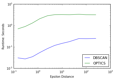
plot(epsilons,eps_times_DB,'b',label='DBSCAN')
plot(epsilons,eps_times_OPT,'g',label='OPTICS')
semilogy()
semilogx()
xlabel("Epsilon Distance")
ylabel("Runtime: Seconds")
legend(loc=4)

<matplotlib.legend.Legend at 0x11133c410>

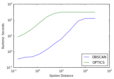
eps_times_DB_40k,eps_times_OPT_40k

([0.3324090639750163,
  0.4331480662027995,
  0.4585415522257487,
  0.6865076224009196,
  1.3512890338897705,
  2.991980711619059,
  6.290017286936442,
  18.496273676554363,
  84.68666569391887,
  121.54244637489319,
  120.43232997258504],
 [8.212754408518473,
  13.50602944691976,
  26.57088589668274,
  65.20482174555461,
  155.14100941022238,
  250.5828684171041,
  302.9867091178894,
  304.2664025624593,
  304.4731384118398,
  298.53870995839435,
  303.42804169654846])

# Varying samples benchmark
eps_times_DB_40k_ = []
eps_times_OPT_40k_ = []
for nsamples in nsample:
    benchmark_dbscan = DBSCAN(eps=5.0, min_samples=nsamples)
    outputDB = average_time(benchmark_dbscan.fit,xyz40k)
    eps_times_DB_40k_.append(outputDB[1])

    benchmark_cluster = OPTICS(eps=5.0, min_samples=nsamples)
    outputOPT = average_time(benchmark_cluster.fit,xyz40k)
    eps_times_OPT_40k_.append(outputOPT[1])

    #print nsamples

plot(epsilons,eps_times_DB_40k,'b',label='DBSCAN')
plot(epsilons,eps_times_OPT_40k,'g',label='OPTICS')
semilogy()
semilogx()
xlabel("Epsilon Distance")
ylabel("Runtime: Seconds")
legend(loc=4)

<matplotlib.legend.Legend at 0x1463a0110>

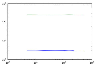
# Varying min_points plot
plot(nsample,eps_times_DB_40k_,'b')
plot(nsample,eps_times_OPT_40k_,'g')
semilogy()
semilogx()

[]

# Varying eps benchmark
eps_times_DB_400k = []
eps_times_OPT_400k = []
for epsilon in epsilons[6:]:
    benchmark_dbscan = DBSCAN(eps=epsilon, min_samples=100)
    outputDB = average_time(benchmark_dbscan.fit,xyz400k)
    eps_times_DB_400k.append(outputDB[1])

    benchmark_cluster = OPTICS(eps=epsilon, min_samples=100)
    outputOPT = average_time(benchmark_cluster.fit,xyz400k)
    eps_times_OPT_400k.append(outputOPT[1])

    print epsilon

eps_times_DB_400k,eps_times_OPT_400k

epsilons[6:]

plot(epsilons[:6],eps_times_DB_400k[:6],'b',label='DBSCAN')
plot(epsilons[:6],eps_times_OPT_400k[:6],'g',label='OPTICS')
semilogy()
semilogx()
xlabel("Epsilon Distance")
ylabel("Runtime: Seconds")
legend(loc=4)