Complex ICESat-2 Queries in the cloud

Although the data referenced in here is stored as columnar parquet files, there is a compatible raster rotation of the tessalation that keeps the same indexing and nesting structure. Tiling 2 and 3 dimensional arrays at defined chunk intervals may be an elegent way for data fusion across gridded and non-gridded large environmental data sets.

Reproducing this notebook

The data in this notebook lives in the cloud, and is ‘free’ to access, in that it does not require payment to me. But it does require an AWS account, and amazon will charge you for compute. The data transfer cost will likely not be noticeable if you are in the US West-2 region where we are hosting it… but might be pricey if you cross regions or try and export it at volume outside of the cloud.

I use an instance with 256GB of ram to run this notebook; the first data pull is ‘small’ at ~20GB in memory. The second pull is over 100GB of memory, and will crash the kernel and dask if you are on too small of a machine. Everything here is under development, but particularly the indexing scheme, which has already changed. The most recent version of healpix morton indexing is at the mortie library… but it produces breaking changes will not work with the data reference in this notebook (i.e., the data already stored in S3), which is why the old functions are replicated instead of imported.

One obvious way to run this as a smaller notebook would be to modify to only grab a single orbital period; as written, this grabs a two year time series for each of the basins.

import vaex

import numpy as np
from numpy import r_
import pandas as pd
import matplotlib.pyplot as plt

import mhealpy as mh
from tqdm.notebook import tqdm

from numba import jit, int64, vectorize

from dask_gateway import Gateway

gateway = Gateway()
options = gateway.cluster_options()
options.worker_specification = '4CPU, 16GB'
cluster = gateway.new_cluster(options)
cluster.scale(32)
client = cluster.get_client(set_as_default=True)
client

Client

Client-00e1c11b-5982-11ed-957e-02fed3e5ba98

Connection method: Cluster object	Cluster type: dask_gateway.GatewayCluster
Dashboard: /services/dask-gateway/clusters/prod.1115cf8cd0e9418283b3a6207e42bb95/status

Cluster Info

GatewayCluster

• Name: prod.1115cf8cd0e9418283b3a6207e42bb95
• Dashboard: /services/dask-gateway/clusters/prod.1115cf8cd0e9418283b3a6207e42bb95/status

Tiling

The mhealpy library is an superset of the healpy library that adds support for multiresolution healpix maps. The astronomy community uses a different indexing scheme then the ‘morton’ ordering used in this notebook. There’s actually three different schemes that are provided for: ring, nested and uniq, with the first two being fixed resolution, and the last being multiresolution.

There are facilities for converting between to representations, and certain index methods are optimized for different types of plotting methods. We use the optimized healpix code, and then convert from nested format to morton indexing.

A few things to note here–

1. The data has already been tiled and uploaded; what is being shown is traversing the morton/healpix embedding space tree to retrieve that data. How to write the data shards is a post for another day.

2. All of the functions in the next cell are out of date; the mortie library has an updated number scheme that fixes several bugs, and marks southern hemisphere data as negative integers. However, the S3 shards were uploading using this previous scheme, so we’re using old functions to index to that data structure.

3. The shard and chunk sizes add 2 levels to the tree. An updated data upload would add an addition tree level for the S3 partitions. The reason will be apparent later on; we’re downloading quite a lot of data for fine scale queries. This would be an even more pronounced issue if this was ATL03 data.

In other words, the next update to this will break the numbering scheme here, change tree depth, and be more amenable to ATL03 data.

# These are old and outdated
def unique2parent(unique):
    '''
    Assumes input is UNIQ
    Currently only works on single resolution
    Returns parent base cell
    '''
    nside = mh.uniq2nside(unique)
    if nside.all():
        order = int(np.log2(nside.max()))
    unique = unique // 4**(order-1)
    parent = (unique - 16) // 4
    return parent

def heal_norm(base, order, addr_nest):
    N_pix = mh.hp.order2nside(order)**2
    addr_norm = addr_nest - (base * N_pix)
    return addr_norm

@vectorize([int64(int64, int64, int64)])
def fastNorm2Mort(order, normed, parents):
    # General version, for arbitary order
    if order > 18:
        raise ValueError("Max order is 18 (to output to 64-bit int).")
    mask = np.int64(3*4**(order-1))
    res = np.zeros(order,dtype=np.int64)
    num = 0
    for j, i in enumerate(range(order, 0, -1)):
        nextBit = (normed & mask) >> ((2*i) - 2)
        num += (nextBit+1) * 10**(i-1)
        mask = mask >> 2
    if parents is not None:
        parents = parents- 6
        parents = parents * 10**(order)
        num = num + parents
    return num

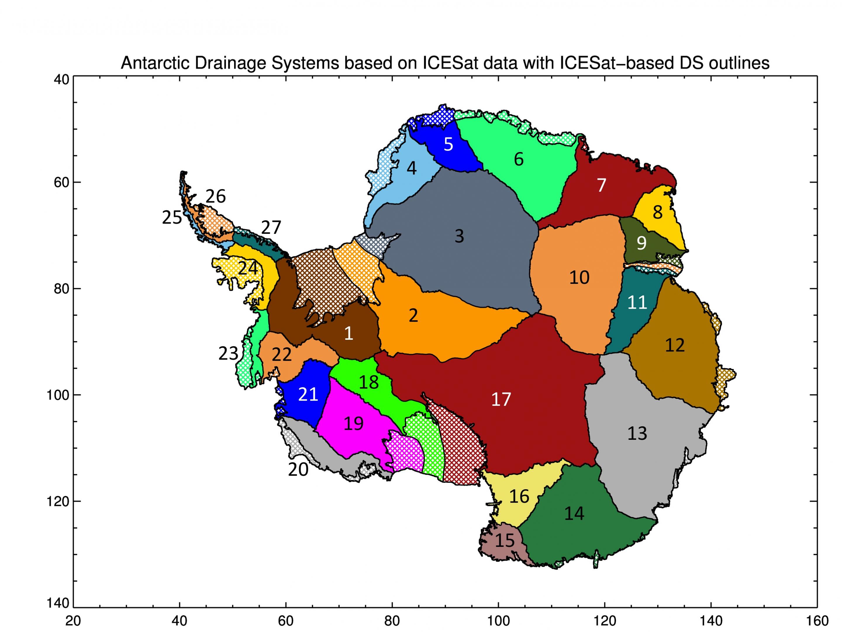
# Read in drainage basin polylines
# Source: http://icesat4.gsfc.nasa.gov/cryo_data/drainage_divides/Ant_Grounded_DrainageSystem_Polygons.txt
basins = pd.read_csv('./Ant_Grounded_DrainageSystem_Polygons.txt',
                     delim_whitespace=True,
                     names = ['Lat', 'Lon', 'basin'])

basins

	Lat	Lon	basin
0	-74.525273	-61.122545	1
1	-74.525435	-61.123664	1
2	-74.525467	-61.123826	1
3	-74.525576	-61.124567	1
4	-74.525609	-61.124498	1
...	...	...	...
1238996	-74.523392	-61.109736	27
1238997	-74.523938	-61.113444	27
1238998	-74.524484	-61.117151	27
1238999	-74.525030	-61.120859	27
1239000	-74.525273	-61.122545	27

1239001 rows × 3 columns

Querying Data

Healpix spatial queries occur seperate from the data; all that we need to do is define the grid cell resolution:

def order2res(order):
    res = 111* 58.6323*.5**order
    return res

for res in range(20):
    print(str(order2res(res))+ ' km at tesselation order ' + str(res))

6508.1853 km at tesselation order 0
3254.09265 km at tesselation order 1
1627.046325 km at tesselation order 2
813.5231625 km at tesselation order 3
406.76158125 km at tesselation order 4
203.380790625 km at tesselation order 5
101.6903953125 km at tesselation order 6
50.84519765625 km at tesselation order 7
25.422598828125 km at tesselation order 8
12.7112994140625 km at tesselation order 9
6.35564970703125 km at tesselation order 10
3.177824853515625 km at tesselation order 11
1.5889124267578125 km at tesselation order 12
0.7944562133789063 km at tesselation order 13
0.39722810668945313 km at tesselation order 14
0.19861405334472657 km at tesselation order 15
0.09930702667236328 km at tesselation order 16
0.04965351333618164 km at tesselation order 17
0.02482675666809082 km at tesselation order 18
0.01241337833404541 km at tesselation order 19

Requesting an ‘order’ of 11 will select grid cells that roughly 3km per side. However, the healpix query only guarantees that the observation is somewhere in that cell; we don’t know if it is at the edge, or at center. Going up one order of resolution doesn’t solve this problem for us– if we want to execute a ‘buffer’, we need to calculate a neighborhood function. Fortunately, the base healpix library provides functions to do this, and we can cast the results to the morton numbering scheme. The neighborhood function will return all of the cells touching cell that the observation is present in, so calling it at order 11 will return a 9km area about the observation location, with a guarantee of at least 3km of buffer in every direction. This is quite fast:

%%time
# Set order
order = 11
# Subset basin 2
b2 = basins[basins.basin == 2]
# Get all nieghbors
B2_11 = mh.hp.pixelfunc.get_all_neighbours(2**order, b2.Lon.values,
                                           b2.Lat.values, nest=True,
                                           lonlat=True)
# Drop repeats
Basin2_11 = np.unique(B2_11.ravel())

CPU times: user 24.6 ms, sys: 0 ns, total: 24.6 ms
Wall time: 20.6 ms

Again, with healpix the query is separate from the data, and we can visualize what our cells will look like, even if we don’t know a priori if those cells actually have anything inside them:

nside = 2**11
m = np.zeros(mh.hp.nside2npix(nside))
m[Basin2_11.ravel()] += 1
mh.hp.gnomview(m, rot=[0,-90], xsize=800, ysize=800, nest=True)

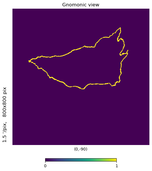
That’s our 3km buffer for basin 2.

Our parquet data is sharded and stored at a different resolution; we can down-sample our result to figure out the S3 paths that we need to download to get the data:

%%time
# Convert to Morton indexing
order = 11
uniq = mh.nest2uniq(2**order, Basin2_11)
parents = unique2parent(uniq)
normed = heal_norm(parents,order, uniq)
# Get 'full' resolution
mortonsB2_11 = fastNorm2Mort(order,normed.ravel(), parents.ravel())
# Degrade to shard resolution
Basin2_6 = mortonsB2_11 // 10**5
Basin2_6 = np.unique(Basin2_6)

CPU times: user 2.28 ms, sys: 0 ns, total: 2.28 ms
Wall time: 1.86 ms

len(mortonsB2_11), len(Basin2_6)

(6106, 64)

# Approximate view of data in S3
nside = 2**6
b2idx = mh.hp.ang2pix(nside,b2.Lon.values, b2.Lat.values, lonlat=True)
m = np.zeros(mh.hp.nside2npix(nside))
m[np.unique(b2idx).ravel()] += 1
# Centered on the south pole
mh.hp.gnomview(m, rot=[0,-90], xsize=800, ysize=800)# , nest=True)
print(len(np.unique(b2idx).ravel()))

60

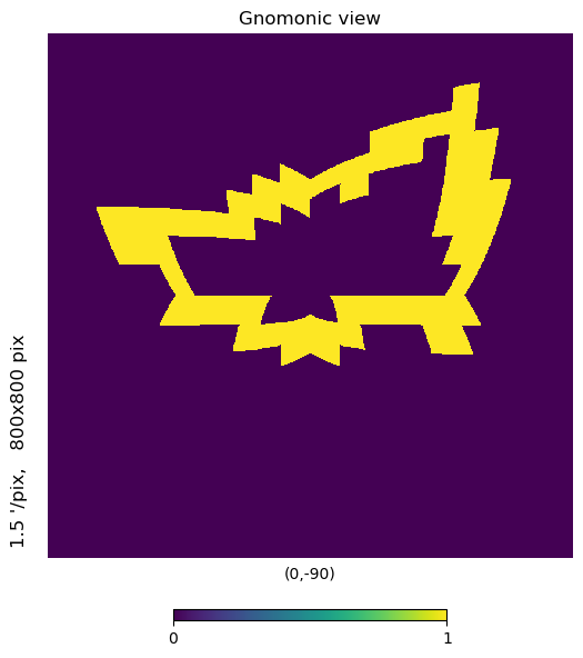
We can see that the basin outline for 3km resolution is split over 6,106 ‘cells’, but those cells are in turn split over 64 parquet files– at most, the pole hole actually results in some empty shards.

You might notice a discrepancy above– there’s 64 parquet files, but the plot above only shows 60 shards plotted. That’s because when we degraded to the shard resolution, we did it off the 3km buffer, which crossed over to a few adjacent cells… 4 of which pushed to adjacent shards. By doing the buffer at the higher resolution we don’t miss any potential points, but also don’t over subscribe to unneeded shards if we did the buffer at the lower resolution.

We can build the file list in a loop, and get the data in parallel on distributed workers:

cycles = ['4','5','6','7','8','9','10','11']
prefix = 's3://geostacks/icesat_2/shards='
mid = '/cycle='
suffix = '/atl06.parquet'

filelist = []

for i in Basin2_6:
    for j in cycles:
        s3path = prefix + str(i) + mid + j + suffix
        filelist.append(s3path)

# 64 shards repeated for years / 8 cycles
len(filelist)

512

We could request all the data be returned using this:

def get_thing_full(s3file):
    return vaex.open(s3file).to_arrow_table()

…but we’ll go one step further and do the subsetting on the workers as well:

def get_thing(s3file, cells):
    df = vaex.open(s3file)
    # Get to our query resolution
    df['midx11'] = df.midx // 10**7
    df['basin2'] = df.midx11.isin(cells)
    df.select(df.basin2 == True)
    tmp = df.to_arrow_table(selection=True, parallel=True)
    return tmp

The next cell will fail if the cluster workers aren’t spun up yet, so it’s good practice to check if they’re online… and to resubmit the scale call if not. The failure is related to the semantics of scatter, which expects to distribute the data to workers at execution time. This is different than client.submit, which will be more than happy to submit jobs to non-existent workers; the jobs will just queue until workers come online without error. For the latter case, sometimes this will actually speed up worker allocation, as ad hoc workers tend to activate faster when they know there is work for them!

client.scatter(mortonsB2_11, broadcast=True)

Future: ndarray status: finished, type: numpy.ndarray, key: ndarray-56609e93e968cc406bde452fcdc64f7d

futures = []
for thing in filelist:
    futures.append(client.submit(get_thing, thing, mortonsB2_11, retries=10))

# ~22GB return
quiver = list(filter(None, client.gather(futures, errors='skip', direct=True)))

big_list = []
for arrow in quiver:
    big_list.append(vaex.from_arrow_table(arrow))

df = vaex.concat(big_list)

df

#	id	lat	lon	slope_y	slope_x	slope_x_sigma	h_li	s_li	q_flag	s_fg	snr	h_rb	bsnow_conf	cloud_flg_asr	cloud_flg_atm	msw_flag	fbsnow_h	bsnow_od	layer_flag	bckgrd	e_bckgrd	n_fit_photons	w_surface_window_final	t_year	track	x	y	midx	shards	cycle	midx11	basin2
0	1523093	-86.14954851360491	33.92593579210944	-0.0395953431725502	0.00046188640408217907	0.0006559690809808671	2939.65185546875	0.012169521301984787	0	0	0.0	0.16256438195705414	6	2	0	4	56.94702911376953	0.07961465418338776	1	23297.232421875	0.0	482	3.0	2019-07-10 02:32:02.307540	gt1l	232881.35931420964	346225.37644100154	2111134242242111122	2111134	4	211113424224	True
1	1523094	-86.14939581927959	33.92457007097016	-0.06023023650050163	-0.006562550086528063	0.0006581993075087667	2939.58447265625	0.01336896326392889	0	0	0.0	0.1646553874015808	6	2	0	4	59.05659103393555	0.08079415559768677	1	25988.84375	0.0	465	3.0	2019-07-10 02:32:02.310355	gt1l	232882.34804547214	346244.66751049814	2111134242242111124	2111134	4	211113424224	True
2	1523095	-86.14924304204673	33.92320645695685	-0.06262587010860443	-0.003759956220164895	0.0007193252677097917	2939.484375	0.013828647322952747	0	0	0.0	0.18167147040367126	6	2	0	4	58.752349853515625	0.08070683479309082	1	27742.94921875	0.0	461	3.0	2019-07-10 02:32:02.313168	gt1l	232883.35374213205	346263.95772095054	2111134242242111142	2111134	4	211113424224	True
3	1523096	-86.14909011053149	33.92184672722354	-0.025539278984069824	0.008118819445371628	0.0006527432706207037	2939.517578125	0.012108918279409409	0	0	0.0	0.16191399097442627	6	2	0	4	56.649208068847656	0.07967527210712433	1	28792.603515625	0.0	475	3.0	2019-07-10 02:32:02.315974	gt1l	232884.39146603562	346283.2462720065	2111134242242111142	2111134	4	211113424224	True
4	1523097	-86.14893700260534	33.92049143181697	-0.03492480516433716	0.011287172324955463	0.0006484501645900309	2939.72021484375	0.012137381359934807	0	0	0.0	0.16041499376296997	6	2	0	4	54.551910400390625	0.07864658534526825	1	24003.869140625	0.0	487	3.0	2019-07-10 02:32:02.318772	gt1l	232885.46588380224	346302.53291968664	2111134242242111144	2111134	4	211113424224	True
...	...	...	...	...	...	...	...	...	...	...	...	...	...	...	...	...	...	...	...	...	...	...	...	...	...	...	...	...	...	...	...	...
116,343,239	1549043	-81.82003381242077	-49.04448300989648	4.835084837395698e-05	0.0017873976612463593	0.0004322136810515076	88.74310302734375	0.007835650816559792	0	0	0.0	0.10365600883960724	-1	2	1	1	29.979246139526367	0.028110453858971596	1	148184.5625	0.0	424	3.0	2021-06-11 21:24:54.182550	gt3r	-670302.7729052545	581772.2705912268	5111432111414434313	5111432	11	511143211141	True
116,343,240	1549044	-81.81986157860989	-49.04480402632936	0.0001920364156831056	-0.0016964105889201164	0.000489795405883342	88.74688720703125	0.007848388515412807	0	0	0.0	0.11242944747209549	-1	2	1	1	29.979246139526367	0.027972066774964333	1	146144.84375	0.0	426	3.0	2021-06-11 21:24:54.185357	gt3r	-670320.1922462292	581780.8045149728	5111432111414434314	5111432	11	511143211141	True
116,343,241	1549045	-81.81968929358989	-49.04512368181247	0.0005683625931851566	0.0004018144973088056	0.0005003189435228705	88.71788024902344	0.009416015818715096	0	0	0.0	0.11978613585233688	-1	2	1	1	29.979246139526367	0.027833567932248116	1	131252.15625	0.0	426	3.0	2021-06-11 21:24:54.188167	gt3r	-670337.6020975797	581789.3578408199	5111432111414434332	5111432	11	511143211141	True
116,343,242	1549046	-81.81951694599303	-49.04544167739985	0.0005571695510298014	0.001968930708244443	0.00044805006473325193	88.7217788696289	0.007712152320891619	0	0	0.0	0.10411503911018372	-1	2	1	1	29.979246139526367	0.027694901451468468	1	128720.234375	0.0	439	3.0	2021-06-11 21:24:54.190980	gt3r	-670355.0003577591	581797.9348786987	5111432111414434334	5111432	11	511143211141	True
116,343,243	1549047	-81.81934457364784	-49.045759009733075	-7.287902553798631e-05	-0.0009209429263137281	0.00045299253542907536	88.7392578125	0.00943058729171753	0	0	0.0	0.11246149241924286	-1	2	1	1	29.979246139526367	0.02755611203610897	1	135125.71875	0.0	458	3.0	2021-06-11 21:24:54.193796	gt3r	-670372.3940364019	581806.5212699741	5111432111414434334	5111432	11	511143211141	True

We can also do the same for all of the basins, and do a 3km buffer for the entire continent:

%%time
# Set order
order = 11
# Get all neighbors
B11 = mh.hp.pixelfunc.get_all_neighbours(2**order, basins.Lon.values,
                                           basins.Lat.values, nest=True,
                                           lonlat=True)
# Drop repeats
B_11 = np.unique(B11.ravel())

uniq = mh.nest2uniq(2**order, B_11)
parents = unique2parent(uniq)
normed = heal_norm(parents,order, uniq)
# Get 'full' resolution
mortons11 = fastNorm2Mort(order,normed.ravel(), parents.ravel())
# Degrade to shard resolution
Basin11 = mortons11 // 10**5
Basin11 = np.unique(Basin11)

cycles = ['4','5','6','7','8','9','10','11']
prefix = 's3://geostacks/icesat_2/shards='
mid = '/cycle='
suffix = '/atl06.parquet'

filelist = []

for i in Basin11:
    for j in cycles:
        s3path = prefix + str(i) + mid + j + suffix
        filelist.append(s3path)

CPU times: user 353 ms, sys: 29.4 ms, total: 382 ms
Wall time: 381 ms

len(filelist)

5432

client.scatter(mortons11, broadcast=True)

Future: ndarray status: finished, type: numpy.ndarray, key: ndarray-45290d95a6ffdfd8d6e31725309b1ea1

%%time
results = []
for thing in filelist:
    results.append(client.submit(get_thing, thing, mortons11, retries=10))

# extra logic for bigger dataset-- start download to host pre-emptively
lst = np.array_split(results, 10)
big_list = []
for thing in tqdm(lst):
    futures = thing.tolist()
    quiver = list(filter(None, client.gather(futures, errors='skip', direct=True)))
    for future in futures:
        future.cancel()
    for arrow in quiver:
        big_list.append(vaex.from_arrow_table(arrow))

CPU times: user 2min 59s, sys: 1min 2s, total: 4min 2s
Wall time: 24min 8s

Slightly different logic for the larger run– we’re chunking the download into 10 partitions, and asynchronously transferring the data back as it completes. This does three things:

1. Avoids brittle behavior in dask, which likes to crash when you start to exceed a dozen or so data GB to transfer in one go

2. Speeds up the computation by allowing us to send results back parallel to additional computation occurring

3. Clears the results off of the workers, which frees memory– this allows us to save money by sizing smaller workers

Note that not only is the download from S3 data stores occurring in parallel, but also the filtering of the subsets is also occurring on the worker for more efficient horizontal scaling.

df = vaex.concat(big_list)

df

#	id	lat	lon	slope_y	slope_x	slope_x_sigma	h_li	s_li	q_flag	s_fg	snr	h_rb	bsnow_conf	cloud_flg_asr	cloud_flg_atm	msw_flag	fbsnow_h	bsnow_od	layer_flag	bckgrd	e_bckgrd	n_fit_photons	w_surface_window_final	t_year	track	x	y	midx	shards	cycle	midx11	basin2
0	1523093	-86.14954851360491	33.92593579210944	-0.0395953431725502	0.00046188640408217907	0.0006559690809808671	2939.65185546875	0.012169521301984787	0	0	0.0	0.16256438195705414	6	2	0	4	56.94702911376953	0.07961465418338776	1	23297.232421875	0.0	482	3.0	2019-07-10 02:32:02.307540	gt1l	232881.35931420964	346225.37644100154	2111134242242111122	2111134	4	211113424224	True
1	1523094	-86.14939581927959	33.92457007097016	-0.06023023650050163	-0.006562550086528063	0.0006581993075087667	2939.58447265625	0.01336896326392889	0	0	0.0	0.1646553874015808	6	2	0	4	59.05659103393555	0.08079415559768677	1	25988.84375	0.0	465	3.0	2019-07-10 02:32:02.310355	gt1l	232882.34804547214	346244.66751049814	2111134242242111124	2111134	4	211113424224	True
2	1523095	-86.14924304204673	33.92320645695685	-0.06262587010860443	-0.003759956220164895	0.0007193252677097917	2939.484375	0.013828647322952747	0	0	0.0	0.18167147040367126	6	2	0	4	58.752349853515625	0.08070683479309082	1	27742.94921875	0.0	461	3.0	2019-07-10 02:32:02.313168	gt1l	232883.35374213205	346263.95772095054	2111134242242111142	2111134	4	211113424224	True
3	1523096	-86.14909011053149	33.92184672722354	-0.025539278984069824	0.008118819445371628	0.0006527432706207037	2939.517578125	0.012108918279409409	0	0	0.0	0.16191399097442627	6	2	0	4	56.649208068847656	0.07967527210712433	1	28792.603515625	0.0	475	3.0	2019-07-10 02:32:02.315974	gt1l	232884.39146603562	346283.2462720065	2111134242242111142	2111134	4	211113424224	True
4	1523097	-86.14893700260534	33.92049143181697	-0.03492480516433716	0.011287172324955463	0.0006484501645900309	2939.72021484375	0.012137381359934807	0	0	0.0	0.16041499376296997	6	2	0	4	54.551910400390625	0.07864658534526825	1	24003.869140625	0.0	487	3.0	2019-07-10 02:32:02.318772	gt1l	232885.46588380224	346302.53291968664	2111134242242111144	2111134	4	211113424224	True
...	...	...	...	...	...	...	...	...	...	...	...	...	...	...	...	...	...	...	...	...	...	...	...	...	...	...	...	...	...	...	...	...
502,554,965	1643664	-65.1595352894234	-64.14736624840631	3.4028234663852886e+38	0.4343118965625763	0.08810029178857803	814.0770263671875	2.443772315979004	1	2	0.0	5.0	127	5	1	3	29.979246139526367	-2.748199462890625	1	95096.1171875	0.0	32	30.0	2021-06-02 22:11:39.206742	gt3r	-2458716.895432818	1191377.9171924246	5134112212142221244	5134112	11	513411221214	True
502,554,966	1643665	-65.1593575757191	-64.14740984828781	3.4028234663852886e+38	-1.3402669429779053	0.09628021717071533	794.2894897460938	2.651156425476074	1	2	0.0	5.0	127	5	1	3	29.979246139526367	-2.748805522918701	1	94514.2890625	0.0	30	34.18221664428711	2021-06-02 22:11:39.209570	gt3r	-2458735.934009656	1191384.8320884425	5134112212142221422	5134112	11	513411221214	True
502,554,967	1643666	-65.15917990299222	-64.14745429112405	0.026572395116090775	0.13136883080005646	0.09426511079072952	778.3578491210938	2.0801053047180176	1	2	0.0	5.0	127	5	1	3	29.979246139526367	-2.749412775039673	1	98183.234375	0.0	25	30.0	2021-06-02 22:11:39.212404	gt3r	-2458754.985957636	1191391.7087620741	5134112212142221424	5134112	11	513411221214	True
502,554,968	1643667	-65.15900240514684	-64.14750247559053	3.4028234663852886e+38	0.4388608932495117	0.06979343295097351	782.5272216796875	1.838956356048584	1	2	0.0	5.0	127	5	1	3	29.979246139526367	-2.750018835067749	1	105618.1640625	0.0	39	30.0	2021-06-02 22:11:39.215232	gt3r	-2458774.0978894485	1191398.4161995882	5134112212142222313	5134112	11	513411221214	True
502,554,969	1643668	-65.15882489514628	-64.14755037468672	3.4028234663852886e+38	0.23369531333446503	0.07562870532274246	785.801025390625	2.3799521923065186	1	2	0.0	5.0	127	5	1	3	29.979246139526367	-2.7506251335144043	1	106303.5546875	0.0	39	30.0	2021-06-02 22:11:39.218061	gt3r	-2458793.2051524017	1191405.1364588912	5134112212142222331	5134112	11	513411221214	True

It’s difficult to describe exactly how computationally complicated the above query is. In plain language, we’ve taken all of the drainage basins borders and applied a ~3km buffer about them, and extracted that data over 8 orbital cycles– two full years of ICESat-2 data. The original data files were time ordered, such that each file was a roughly north/south transect going to or from the pole. Because the drainage basins span the full continent and are complex polylines, it’s hard to tell how many ICESat-2 data granules they touch… but a good estimate would be most (i.e., well over half) of them. There’s ~4,000 hdf5 data files per 91-day orbit repeat that covers Antarctica, so for 8 orbit repetitions we can safely assume over 10,000 files having data in them related to this query, although I suspect it’s likely even more files. Of course, you’d need a way to execute the metadata query to know which ones to open; or you’d need to inspect all 16,000 of them.

Above we’ve subset a half billion data points from a set that was over 10 billion, culling through a few terabytes of data to retrieve the ~100GB that we actually care about. Run times vary, but seem to be between 15 and 30 minutes, although one run finished in under 10.

nside = 2**18

def convertcoords(lon, lat):
    healp = mh.hp.ang2pix(nside, lon, lat, nest=True, lonlat=True)
    return healp

# Convert locations to healpix
df['nest'] = df.apply(convertcoords, arguments=[df.lon, df.lat])

# Takes a bit of time to process the nest coordinates for the next few plots...
# ...it is a billion numbers to convert!
nside = 2**18
m = np.zeros(mh.hp.nside2npix(nside))
m[df['nest'].to_numpy().ravel()] += 1

# Showing the Antarctic Peninsula where
# ICESat-2 is within 3km of the basin boundary
mh.hp.gnomview(m, rot=[-50,-75], xsize=800, ysize=800, nest=True)

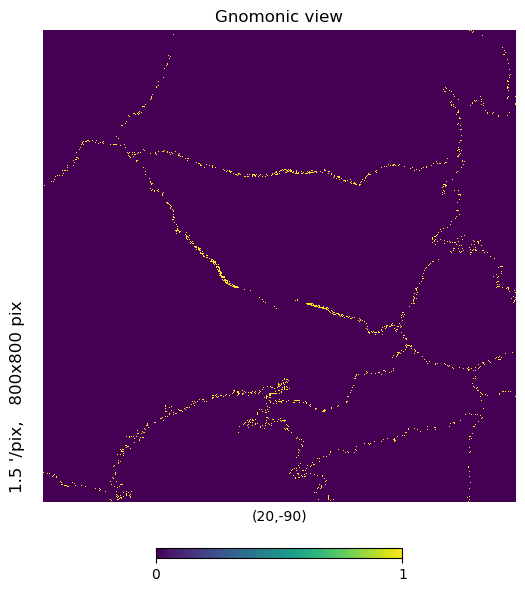
# More inland, by basins 2 and 18, same zoom
mh.hp.gnomview(m, rot=[20,-90], xsize=800, ysize=800, nest=True)

# Higher zoom to see more detail
mh.hp.gnomview(m, rot=[20,-90], xsize=500, ysize=500, nest=True)

That thin band in the center adjacent to dense observation coverage is actually the pole hole. Why are there observations in the hole? Because the first orbital cycle had pointing issues and wasn’t looking nadir for a few overpasses and partially filled it in…

# half a billion points, sparse over the continent
mh.hp.gnomview(m, rot=[0,-90], xsize=1800, ysize=1800, nest=True)

Next Steps

Healpix, and by extension morton ordering, does one thing exceedingly well– it separates the searching of space from the searching of data… although if you store your data using the morton numbers as your directory and file hierarchy, you are effectively doing both.

The morton indexing here sits on a software stack; JPL maintains the base compiled distribution of the healpix library, which is written mostly in fortran and C/C++. Healpy serves as the primary interface (and documentation source), wrapping the numeric routines in python, and providing numerous convenience functions. The mhealpy library provides support for multiresolution functions– especially plotting. Finally, the mortie library that I’ve been developing brings morton indexing which casts the ‘nest’ and ‘unique’ orderings as a more intuitive Hilbert space filling curve that combines both the resolution and location of each address into a single number.

The base JPL library provides fast conversion routines, and also three search methods:

1. Neighbor query. This is what we use in this notebook to make sure our buffer is valid and not missing data by chance.

2. Disk query, in radians. Not shown, but a very common spatial indexing operator.

3. Polygon query

Sadly, the last of these query methods is less robust than I had originally hoped. There are constraints, specifically, that the query polygons need to be convex. This makes the function much less useful, serving potentially as a fast preprocess filter at the cost of additional code complexity. There seem to be two potential fixes– first is in vaex, which has methods for checking for point in polygon. Since vaex is multithreaded by default, and handles large amounts of data well, this is probably the quickest way to enable complex polygon query. I will post a follow up notebook that investigates this functionality, although it will likely be suboptimal in the polar regions if it assumes Euclidean geometry (which most point in polygon algorithms do).

The second option is that the morton reference paper mentions a polygon query method distinct from the base healpix routine. It is not clear to me if the algorithm avoids the non-convex restrictions of the JPL implementation, but it is certainly worth exploring. I am also convinced that the adjacency relations mean that there is a recursive algorithm to fill in the polygon in a fast and efficient way– at the expense of not allowing any ‘holes’ or ‘multipart’ polygons, which seems like a reasonable trade off.

Of course, the more immediate things to do are to update the indexing schema to match the new release of mortie, add the additional level to the tree depth, and experiment with ingesting the much larger ATL03 data.

Previous: Cloud Masking in python using VIIRS